Reconstructing Faraday Waves

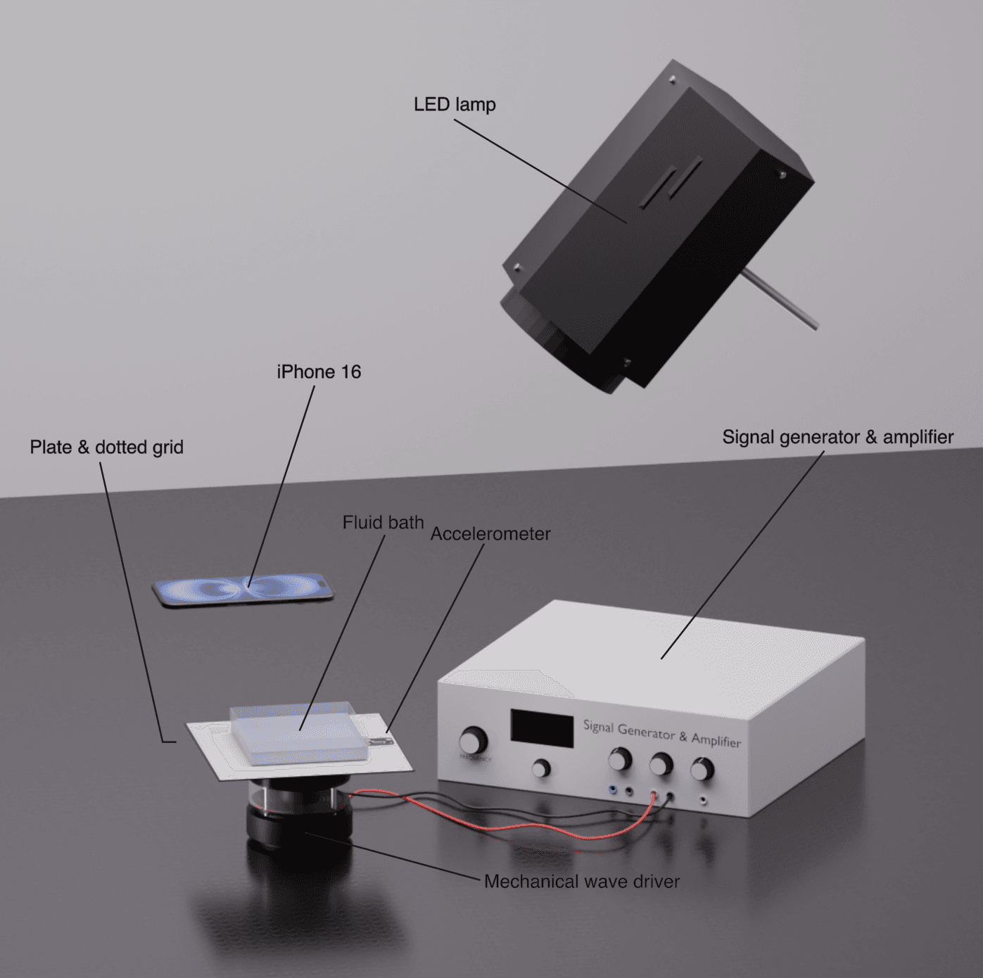
If we want to infer a wave from optical distortion, what must the experiment record? We need the forcing applied to the bath and a stable visual reference beneath the liquid. We therefore place the bath on a mechanical driver controlled by a signal generator and amplifier. An accelerometer measures the imposed vertical motion, while a top-down phone camera watches an opaque grid of dots spaced one millimetre apart beneath the transparent base.

We need three kinds of recording. A stable video is captured after the driving frequency and amplitude have been held fixed long enough for the wave pattern to settle; it supplies the temporal and spatial measurements. A run-up video begins at negligible forcing and continues while we slowly increase the shaker amplitude; it lets us locate the point at which waves begin. Finally, a flat-liquid reference records the undriven bath with its surface flat, giving us the undistorted dot positions for that batch.

As the surface tilts, its local normal redirects a camera ray through the liquid and solid layers, so the corresponding dot appears to move. That apparent shift is our observable: after calibration it will tell us the local surface slope, but it does not yet give us height.

Before we can say that a dot has moved, we need to know where it was before the wave existed. For each batch, we therefore prepare one flat-liquid reference. The toolkit samples frames from this recording and takes their pixel-wise temporal median, which suppresses transient motion and glare. This gives us a stable image from which we can choose a region of interest defined by its centre, dimensions, and rotation.

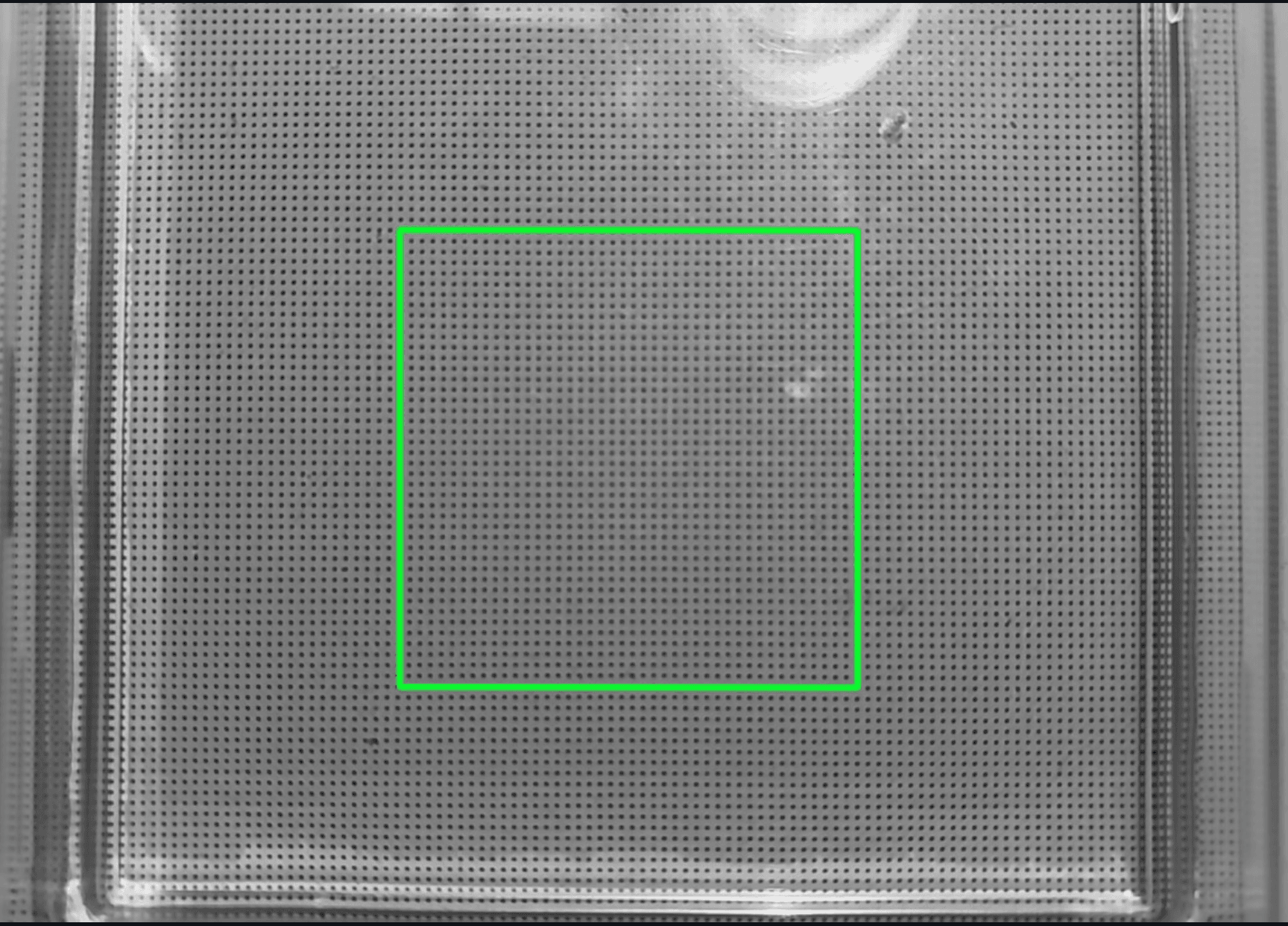
How large should that region be? More dots improve spatial coverage only while they remain individually visible and geometrically reliable. Phone-camera distortion grows toward the edge of the frame, and reflections can hide local groups of points. A smaller central region with nearly uniform spacing is therefore more useful than a larger crop containing more dots but less trustworthy geometry.

The reference still lives in camera pixels, so how do we later recover physical distances? We perform camera calibration from a separate checkerboard recording. OpenCV detects the checkerboard corners across many clear views and estimates the camera matrix and lens distortion. Frequency and onset can remain in pixels, but FSSS needs this calibration together with the known one-millimetre dot spacing to recover physical positions and wavelengths.

We also need the drive that the bath actually experiences, not merely the value entered into the signal generator. The accelerometer supplies that measurement. Because the bath acceleration is approximately sinusoidal, fitting it gives the measured drive frequency $a(t)\approx\Gamma\cos(2\pi f_dt+\delta)$. Here, $a(t)$ is the fitted dimensionless vertical acceleration at time $t$, $\Gamma$ is its amplitude, $f_d$ is the measured drive frequency, and $\delta$ is the phase offset. When a stable sinusoidal fit underestimates the amplitude, the signal envelope provides the corresponding dimensionless acceleration estimate. We now have a stable reference, calibrated geometry, and the measured forcing; the remaining problem is to give every dot an identity and follow its motion.

A stable reference image is useful only if we can turn its optical texture into dots with persistent identities. How do we identify the grid without losing its structure wherever glare hides a point? The three views below show the solution: raw texture becomes a separable dark-dot signal, then an indexed lattice whose neighbours preserve the missing point's place.

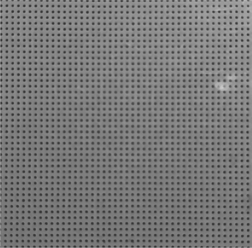
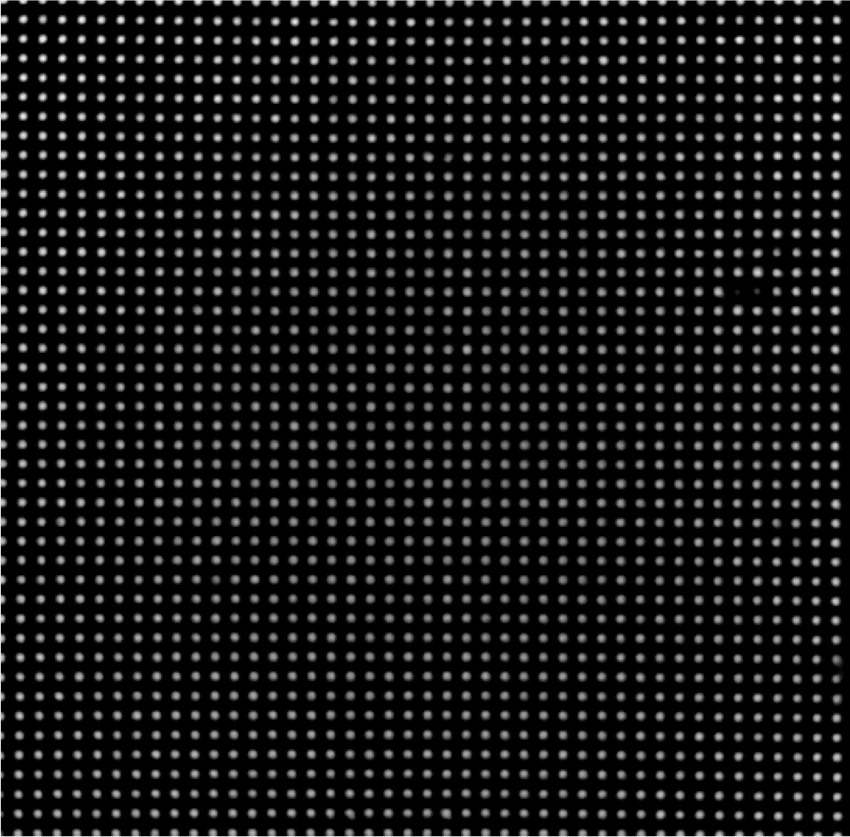
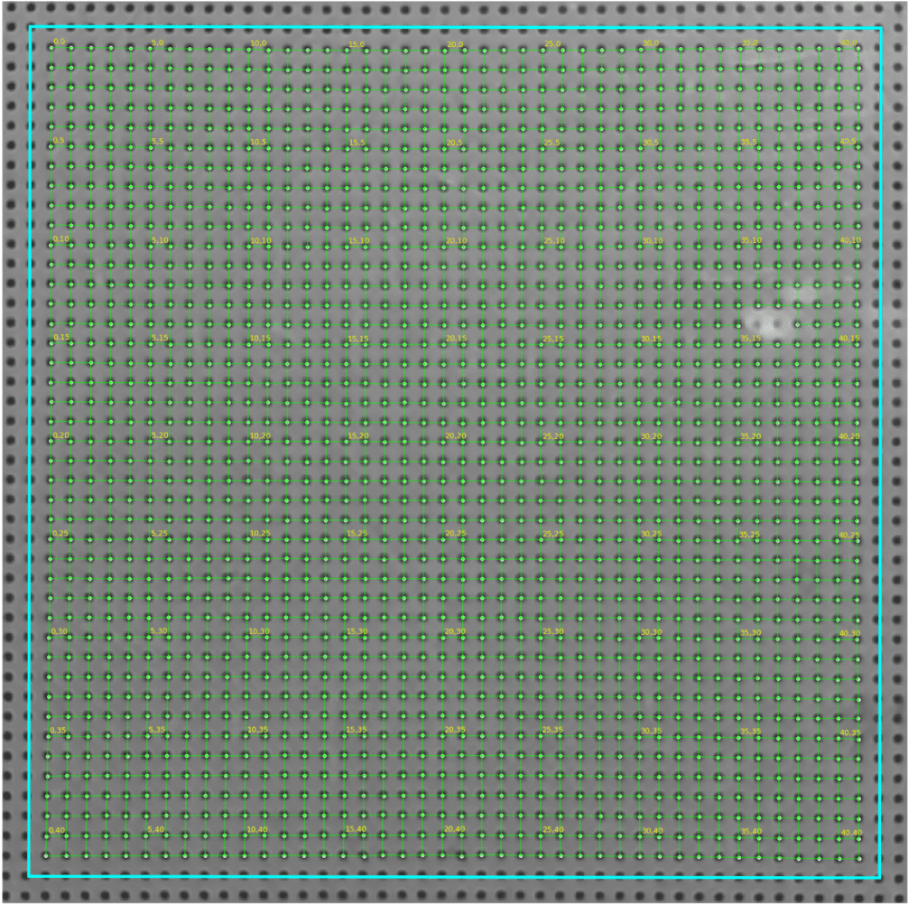
We begin by making each dot easier to separate from the background. Difference-of-Gaussians filtering increases the contrast of the dark features, Otsu thresholding divides those features from the surrounding image, and connected-component analysis reduces every detected blob to a single centre.

Centres alone are still anonymous, so we next ask how each one fits into the known grid. A nearest-neighbour search finds points separated by approximately one grid spacing. Their relative displacement tells us whether a neighbour lies left, right, above, or below, allowing the integer lattice index to propagate from one anchor across the grid. A missed detection around a reflection therefore leaves a gap rather than destroying the identities around it.

Once each reference dot has an identity, how do we follow it through the video? In every later frame we search a small window around its expected position with template matching, rather than detecting and indexing the complete grid again. The correlation maximum gives the moved position and is refined below pixel precision. Its difference from the corresponding flat-reference position is the apparent displacement.

Not all apparent motion comes from the wave. The bath and camera can translate, rotate, or slightly rescale the complete field. We estimate this shared affine motion with RANSAC and subtract it from every measured dot displacement:

Here, $\Delta\mathbf r_{\mathrm{measured}}$ is the tracked dot-displacement vector, $\boldsymbol{\delta}_{\mathrm{affine}}(x,y)$ is the global displacement estimated at image position $(x,y)$, and $\Delta\mathbf r_{\mathrm{corrected}}$ is their residual. What remains is the apparent motion attributed to refraction by the waves. This correction is still an assumption: real wave motion that resembles a global affine transformation can be reduced together with the unwanted camera motion. With a corrected displacement history for every dot, we can now ask what temporal frequencies that collective motion contains.

Tracking tells us where every dot moves, but it does not yet tell us how quickly the surface oscillates. How can we extract the frequencies shared by the complete grid? We start from the affine-corrected displacement in $x$ and $y$ for every indexed dot over time. For a stable video, we centre each trajectory by subtracting its temporal median and remove the frame-wide mean motion. We then apply a Hann window so the beginning and end of the recording contribute less strongly and do not leak as much power into neighbouring frequencies.

We can now test one candidate frequency at a time by projecting the centred motion onto a complex oscillation. If the candidate matches the recorded motion, its contributions add coherently through time; if it does not, they tend to cancel. Both displacement directions can be written compactly as:

The subscript $i$ labels one of the $N$ tracked dots, $t$ is sampled time, $f$ is the tested frequency, $w_t$ is the Hann weight, and $\widetilde{\mathbf u}_i(t)$ is the centred, drift-corrected displacement vector. The roman $\mathrm{i}$ in the exponential is the imaginary unit. The complex projection $\mathbf C_i(f)$ contains the $x$ and $y$ amplitudes of one dot; squaring its magnitude and averaging over the grid gives the spectral power $P(f)$. A high value means that the tested frequency is strongly represented in the collective dot motion.

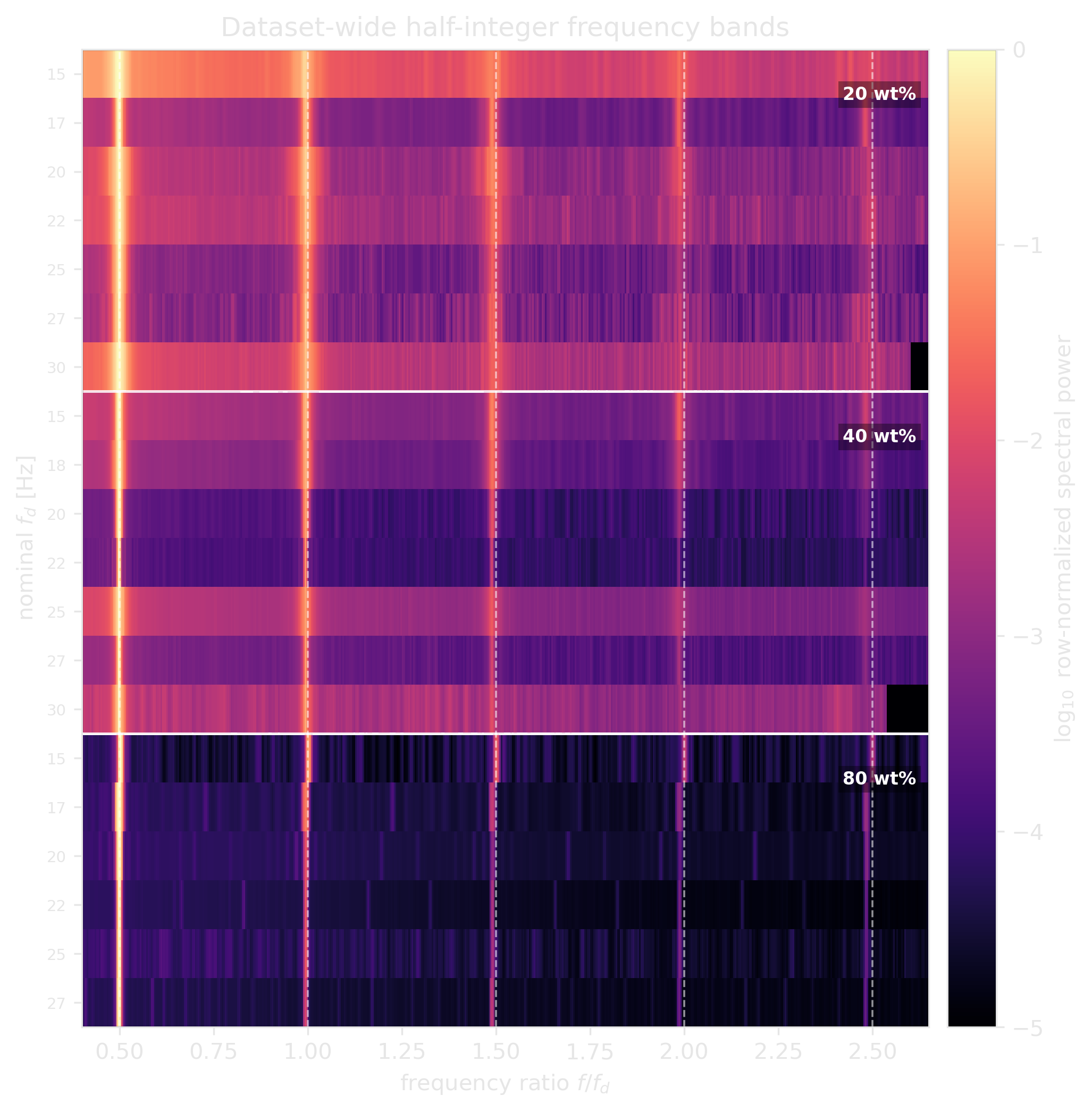
Because the moving surface slope bends the light, its oscillation appears in the motion of the dots. Scanning the candidate frequencies therefore reveals the temporal response of the wave. Faraday-wave theory predicts that the primary response will be subharmonic: it oscillates at half the measured drive frequency. It also predicts frequency bands at successive half-drive intervals—response-to-drive ratios of one-half, one, three-halves, and so on. That is the structure we recover across the dataset: repeated peaks appear at these half-integer intervals, and the half-drive response is usually dominant. The measured frequencies therefore agree with the temporal response expected from theory. We can identify that response—but this still leaves a new question: at what forcing does it first begin to grow?

Now that we can extract the relevant frequencies from the dot motion, how do we know when the waves actually begin? The onset is the forcing threshold at which the initially flat surface becomes unstable and a sustained wave response begins. We locate it from a run-up video, in which the shaker amplitude increases gradually. The accelerometer tells us how strongly the bath is being driven, while the tracking pipeline gives us the dot motion at the same time. Instead of assigning one spectrum to the complete recording, we evaluate the half-drive spectral power in a moving time window, producing a subharmonic envelope through time.

Near the instability threshold, theory predicts exponential growth in that subharmonic response. To connect this growth to the applied forcing, we analyse the accelerometer over the same sequence of short windows. Once the two recordings are synchronized, spectral power and dimensionless driving acceleration share one time axis.

How do we locate the beginning of the growth rather than merely seeing that it happened? We plot the square root of the half-drive power as an amplitude envelope and inspect it on a logarithmic scale. An approximately exponential increase then becomes an approximately straight segment. We manually choose the beginning of that segment as the onset time and read the synchronized acceleration at the same moment:

Here, $t_{\mathrm{onset}}$ is the manually selected onset time, $\Gamma(t)$ is the synchronized dimensionless acceleration trace, and $\Gamma_z$ is the acceleration read from that trace at onset.

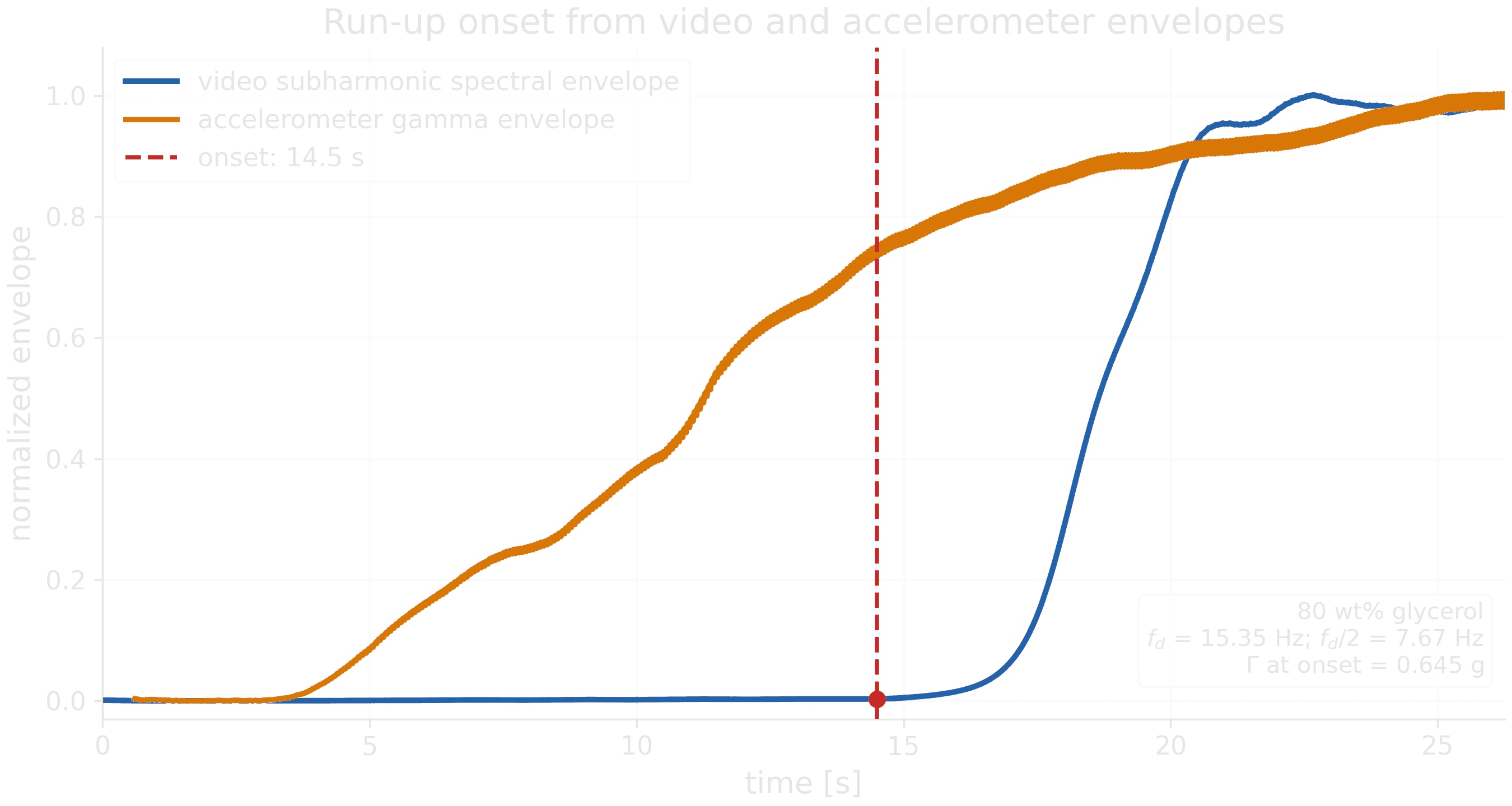
This remains a guided measurement, not an automatic detector. The beginning of linear growth is not perfectly sharp, and the measured onset values were systematically high relative to the theoretical prediction. The toolkit therefore prepares the synchronized evidence while the final onset time remains a human-reviewed choice. Temporal information alone cannot reconstruct the shape of the surface, so the next step is to translate optical displacement into physical slope.

Frequency and onset only require us to compare motion in camera pixels. Reconstructing the surface asks a harder question: what physical slope produced each apparent dot displacement? Free-surface synthetic schlieren (FSSS) answers this by modelling the light rays refracted by the interface. It relates the observed dot motion to the surface gradient, which we can later integrate into height.

The quantity we need from calibration is therefore a matrix that converts apparent displacement in the physical grid plane into surface slope:

Here, $\zeta(x,y)$ is surface height at physical position $(x,y)$, $\nabla\zeta$ is its two-component gradient, $\Delta\mathbf r_{\mathrm{obj}}$ is apparent displacement on the physical grid plane, and $\mathbf B$ is the fitted two-by-two displacement-to-slope matrix.

Before that matrix can be fitted, the image grid must become a physical plane. We assign every indexed dot its known one-millimetre spacing, giving

In this plane, $i$ and $j$ are integer lattice indices, $d$ is the one-millimetre dot spacing, and $(X,Y,Z)$ are physical grid coordinates with $Z=0$. The camera calibration and these 3D grid coordinates give the camera pose through a PnP solve. A homography then maps flat-liquid pixel positions into millimetres on the physical grid plane. We can now express the tracked motion as the physical apparent displacement required by the FSSS transformation.

But what slope should correspond to a given physical displacement? We cannot answer that from the flat experiment alone, so we model the complete optical stack: air, liquid, a three-millimetre acrylic plate, and a two-millimetre polystyrene bottom, each with its depth and refractive index. We then generate synthetic sinusoidal surfaces whose gradients are known analytically:

Here, $A$ is the prescribed surface amplitude, $k$ is its spatial angular frequency, $\phi$ is phase, $s$ is position along the chosen wave direction, and $\nabla s$is that direction's unit vector. For each synthetic surface and physical dot, ray tracing asks which point on the surface must refract a camera ray so that it reaches that dot through the complete optical stack. We solve the same geometry for a flat surface and subtract the two apparent positions. Each successful ray then gives us the pair we were missing: a known refractive displacement and the analytical gradient that caused it.

We repeat this across many dots, directions, wavelengths, phases, and amplitudes, then solve for matrix $\mathbf B$ by least squares. Calibration has now converted the optical question into a usable rule: for this camera and layer geometry, every measured refractive displacement maps to a physical surface slope.

Calibration gives us local slope, but the surface we want is a height field. How do we recover height from thousands of scattered gradients? For every frame, the homography first converts the tracked positions from pixels into physical coordinates on the grid plane. Relative to the flat reference, these become metric dot displacements, and matrix $\mathbf B$ converts each displacement into the two components of the local surface gradient.

Those slopes are measured only where dots exist. To connect them into one surface, we interpolate them onto a regular grid and use the fact that the height difference between neighbouring points should equal the slope between them multiplied by their separation:

Here, $\zeta_{i,j}$ is height at grid index $(i,j)$; $p$ and $q$ are the measured $x$- and $y$-gradient components at the indicated edge midpoints; and $\Delta x$ and $\Delta y$ are the regular grid spacings.

No single path through noisy slopes will close perfectly, so how do we choose one consistent surface? Collecting all neighbouring differences creates an overdetermined linear system. We solve it as a two-dimensional least-squares problem, choosing the height field whose finite differences best reproduce both measured gradient components:

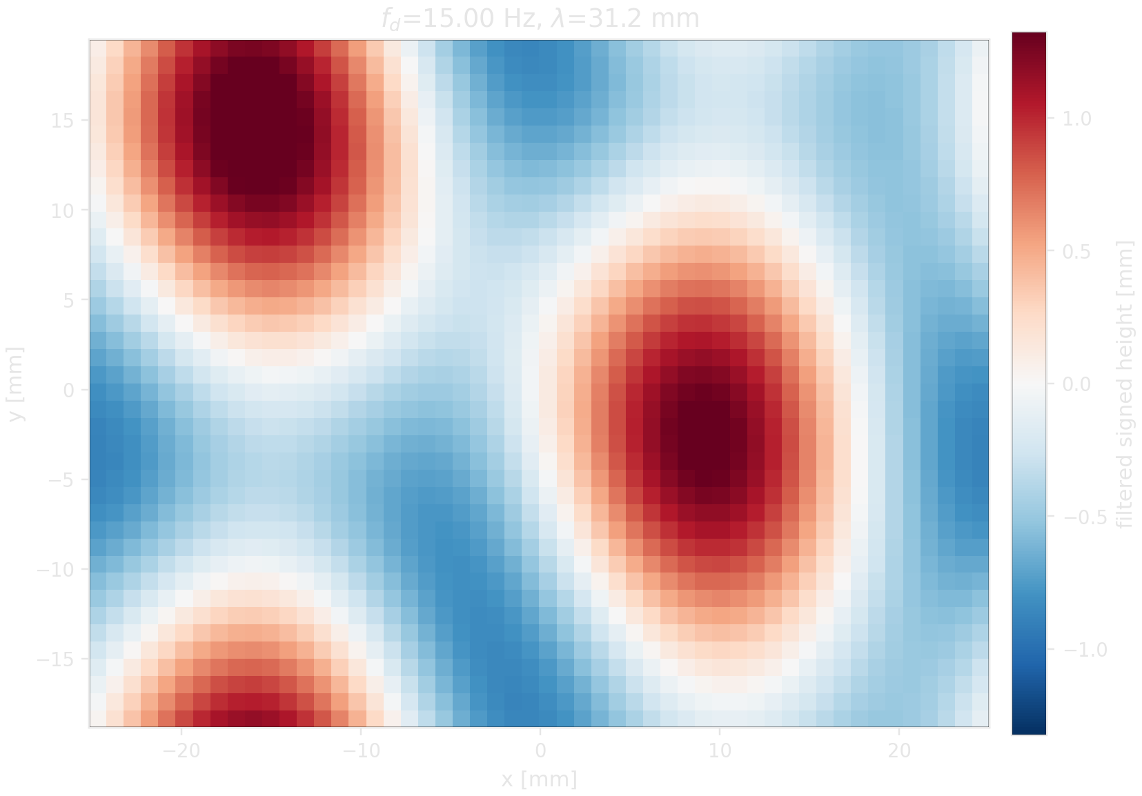
The operators $D_x$ and $D_y$ take finite differences of the unknown height field $\zeta$, while $p$ and $q$ collect the two measured gradient fields; each squared $\ell_2$ norm measures their residual mismatch. Solving this system for every frame produces the signed height map of the evolving surface. The gradients cannot determine an absolute vertical offset, so we interpret the reconstruction relative to its mean height. We can now see the surface through time; the final question is how to turn that changing geometry into a wavelength and spatial mode.

A reconstructed surface still contains many peaks and troughs. Which spatial scale organizes that pattern? We now analyse the height map in space rather than time. For each frame we remove its mean and best-fit plane, apply a two-dimensional Hann window, and transform the surface into a map of spatial Fourier amplitude:

Here, $A(x_n,y_m)$ is the detrended, windowed height at physical sample $(x_n,y_m)$; $m$ and $n$ index the $M$ by $N$ grid; $k_x$ and $k_y$ are the tested wavenumber components; $A_{\mathrm{FT}}$ is their complex spatial amplitude; and the roman $\mathrm{i}$ is the imaginary unit. The coordinates of the dominant peak give the horizontal and vertical wavenumber components. Together they define the dominant wavelength $\lambda$ of the reconstructed standing wave and its scalar wavenumber $k$: $k=\frac{2\pi}{\lambda}$.

Repeating this analysis across driving frequencies lets us ask how the selected pattern changes with the forcing. The signed maps preserve whether the surface lies above or below its mean, while the half-drive power maps emphasize persistent standing-wave nodes: locations that remain near the mean height while the surrounding surface oscillates.

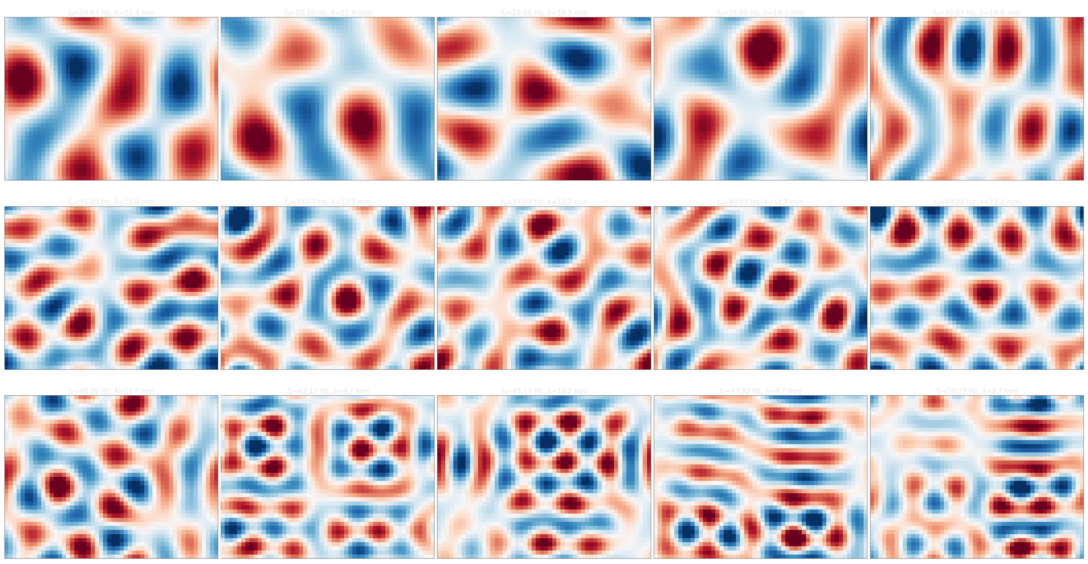
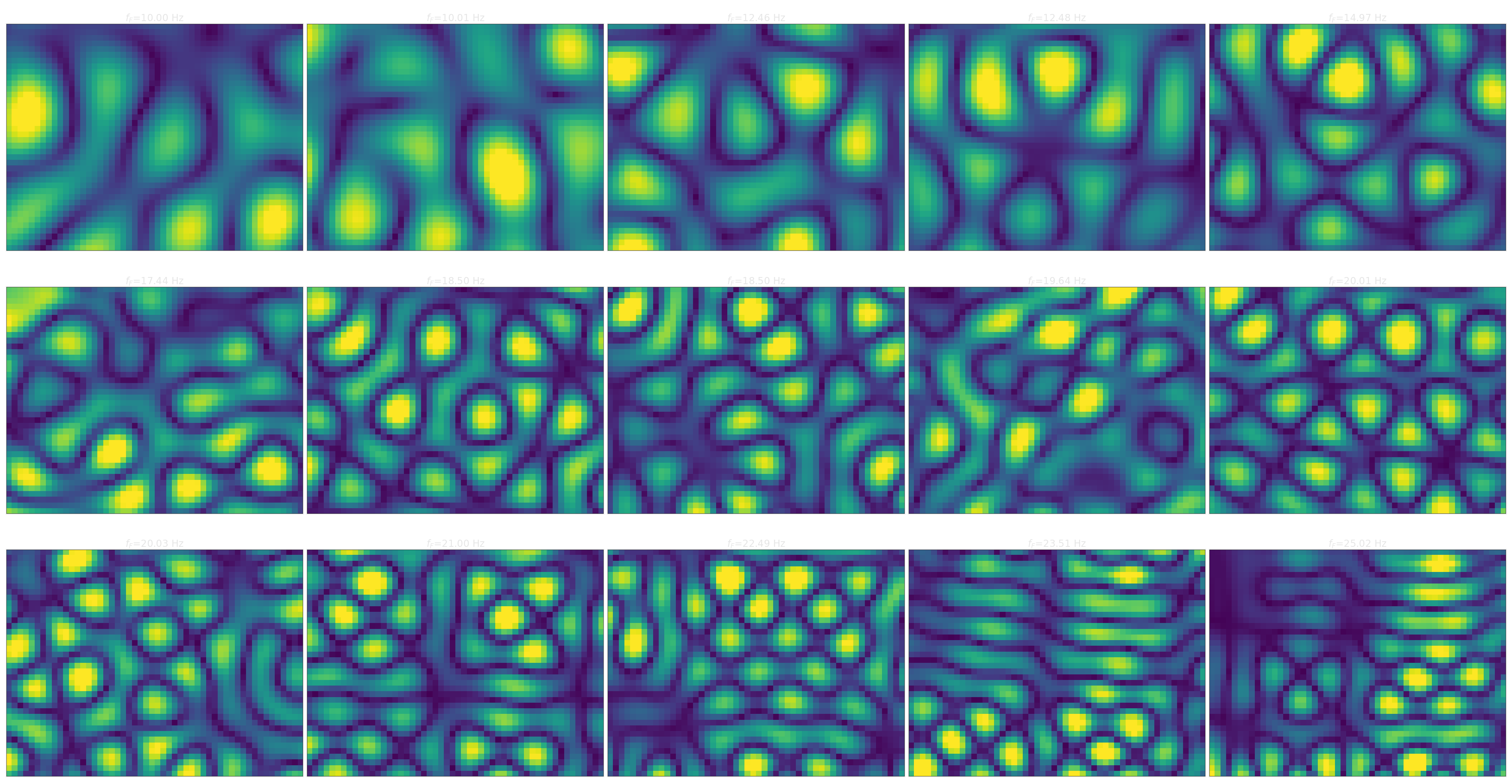
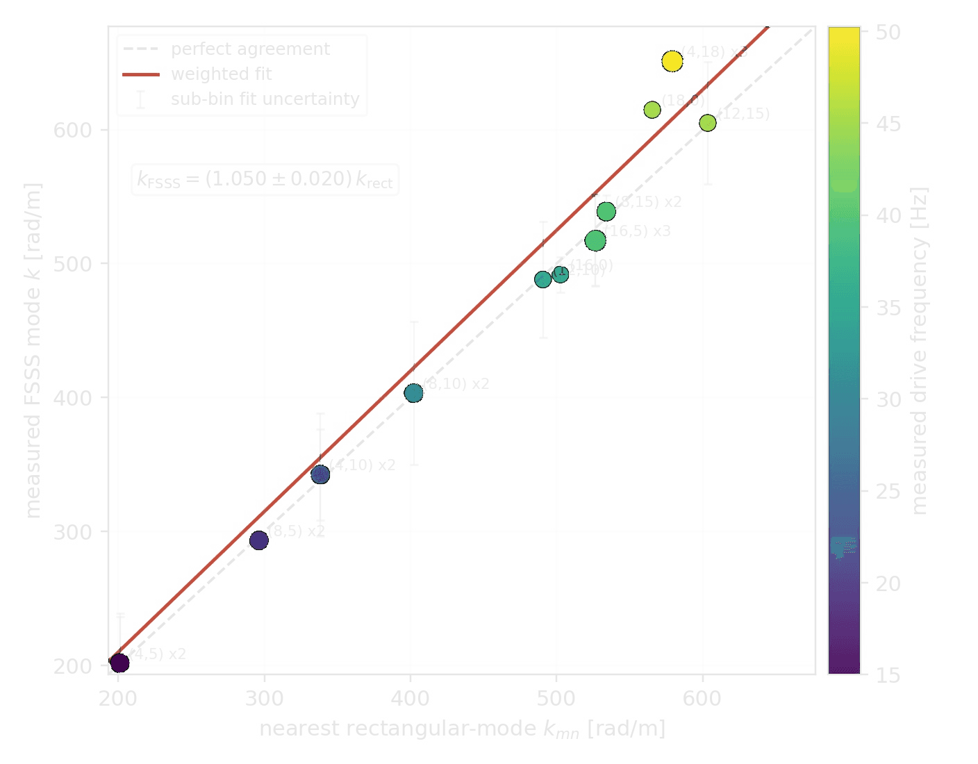
Do the measured patterns agree with the modes allowed by the rectangular bath? A spatial mode is a standing-wave pattern whose wavelength and orientation are compatible with the bath boundaries. The report compares every reconstructed wavenumber with the nearest mode permitted by the rectangular geometry. A fit slope of one would mean that measured and permitted wavenumbers agree one for one; our weighted fit has a slope of $1.050\pm0.020$, close to the ideal value. This supports the boundary-selected mode structure expected for a rectangular bath. The plotted comparison and half-drive height-power maps use the report's processed results; the public toolkit reproduces the underlying reconstruction and Fourier-grid peak. This completes the measurement chain, but it is useful only if we can run it consistently on the rest of the recordings.

How do we make this chain repeatable rather than treating every figure as a one-off analysis? The public Python toolkit packages the Appendix B sequence into three workflows: temporal spectra for stable videos, synchronized onset review for run-up videos, and full FSSS reconstruction for surface height and wavenumber. Each workflow reuses the indexed reference and stores its configuration with the processed result, so a figure can be traced back to the relevant recording and calibration.

The result is not a black box but the same sequence we have just built: establish the reference, track displacement, choose the relevant temporal measurement, calibrate refraction, reconstruct height, and inspect the spatial spectrum. The source code contains the complete implementation and generated artifacts, while the lab report gives the scientific context, derivation, and results.